Leg Design:

December 17, 2016/in Velociraptor (Th), Velociraptor Generation #3/by Paul Ahumada

By: Victoria Osaji, Manufacturing and Development Engineer

Table of Contents

Introduction:

The legs are one of the most important and complicated parts of this project. I mean without legs or not being able to control the robot the project would not meet a lot of requirements and it would not work. So we took this very seriously.

Level 2 Subsystem below:

14. 3rd Generation Velociraptor (Th) shall have a leg design that can support the mass at 505.5g at different positions for standing, bent, and crouching.

Design 1:

Figure 1: This design was modeled after the UCI linkages.

These legs were the image in Figure 1. At first I was having trouble designing these legs because I didn’t understand completely how they worked. But as I did more research, I realized the UCI linkages were all about the circular motion Click Here.

Figure: The model for design 1.

Understanding that, I found a design to reference online. The reason we did not use these legs is because I was having issues simulating the walking pattern on solidworks, I am not sure if there was too much or too little traction. So I decided to 3D print it just to see if I can fix the issue manually. I think the problems stem from the dimensions and the sizing of the legs. I didn’t have any exact measurement, I just eyeballed it and you cannot do that with these robots because they are very sensitive in that sense. Fabian, the President of the Wednesday class, tried to improve this design by making his own. The appearance was better when I simulated it on solidworks the walking pattern was inversed. To conclude, we were unable to use this design.

Design 2:

The next design I modeled on solidworks also was the Theo Jensen model.

Design 3:

This design was also modeled after a model I found on youtube, the Stephenson. For this model I printed out screenshots of the legs from online and measured out every part so I could recreate them on solidworks. The legs consisted of different size triangles, 4 links and 1 one oddly shaped piece plus the foot . The holes for all the connections were 3mm. These legs actually moved on solidworks however they were not doing the complete walking motion so I 3D printed them to manually play with them and I noticed the same thing.

References:

http://sites.uci.edu/markplecnik/projects/leg_mechanisms/

Gear Train:

December 17, 2016/in Velociraptor (Th), Velociraptor Generation #3/by Paul Ahumada

By: Victoria Osaji, Manufacturing and Development Engineer

Introduction:

The mechanical system we implemented was the gear train and it was designed to move the legs, head and tail. For the legs, the small gears have 10 teethes and big gears have 16 teethes. One of the small gears is actually a motor coupler as well that connects to the GM9 motor that will then drive the other gears to move.

Level 2 Subsystem below:

8. 3rd Generation Velociraptor (Th) shall control the head and tail movement with a single servo using gear trains.

11. 3rd Generation Velociraptor (Th) should control the body platform movement with a single servo using gear trains.

Motor Calculations:

To conclude, we will use 56 RPM at 3.7 Volts to drive the small gears to big gears. Since we have 35 RPM, (35RPM/60sec) =0.583 cycle per second for the big gears.

References:

http://www.engr.ncsu.edu/mes/media/pdf/gears

Fall 2016 Velociraptor (W): PCB Layout

December 17, 2016/in Velociraptor (W), Velociraptor Generation #2/by LamNguyen

By: Aaron Choi (Manufacturing Engineer)

Edited and Approved by:

– Lam Nguyen (Project Manager)

– Tim Haddadian (Division Manager for Manufacturing Engineer)

Table of Contents

Requirements

L 1-9 requirement states the Velociraptor shall have an external PCB with an I2C interface which will be similar to the 3DotBoard

Introduction

To fulfill the Level 1-9 requirement, a layout of a custom PCB with Surface Mount Technology (SMT) discrete components will be implemented. This layout will be created through EagleCAD. Once the layout is carried out, approval must be given from Professor Hill or the class President Fabian Sasuke.

Design

The design of the PCB layout revolved around the physical dimensions of the 3DotBoard. The idea is to place the custom PCB above the 3DotBoard. Female pin headers of the PCB will connect to the male pin headers on the 3DotBoard. The battery of the 3DotBoard limits the vertical distance from the PCB to 3DotBoard. This would affect the type of pin headers and connectors used. To avoid the physical constraints, the PCB shall have an L-shape, leaving room for pin header connections to connect properly.

Diagram 1: The figure above shows the SolidWorks model of our PCB.

For the placement and wiring components, rules were carried out following guidelines and tutorials from SparkFun [1] and Professor Hill’s PCB training [2]. The wires were set to a 45 degree angle, the decoupling capacitors were placed close to the IC components, and none of the wiring overlaps.

The placement of the IC components were prioritized on the top layer. The reason for this was to utilize a SMT solder paste stencil for only the top layer. However, due to wiring, one of the IC components were placed on the bottom layer. The IC component placed on the bottom layer shall be hand soldered and utilizing a heat gun. The parts list chosen are given in Table 1 below.

Table1: Parts list ordered from DigiKey.

The final PCB layout is given below.

Diagram 2: The Top Layer wiring of the custom PCB.

Diagram 3: The Bottom Layer wiring of the custom PCB.

Conclusion

Diagram 4: PCB layout with ground planes.

Diagram 4 shows the final PCB layout for the custom PCB design. The custom PCB will be powered by 7.4V external Li-Po batteries. To bring down the voltage, a LDO was incorporated within the PCB. Stepper motor drivers were implemented for the linear actuators, which are micro stepper motors. The connectors for the IMU MPU-6050 were pin headers so that the MPU-6050 can simply be connected to the pin headers without any soldering. After running the Design Rule Check (DRC), no errors were found. The PCB will be ordered from OSH Park and an OSH Park DRC will be carried out.

References

[1] https://learn.sparkfun.com/tutorials/using-eagle-board-layout

[2] http://web.csulb.edu/~hill/ee400d/Technical%20Training%20Series/11%20PCB%20Layout%20with%20Eagle%20CAD%20(Working%20Stencil%20Addition).pdf

IMU System Incorporation

December 17, 2016/in Velociraptor (Th), Velociraptor Generation #3/by Paul Ahumada

By: Paul Ahumada, Systems Engineer

By: Kevin Armentrout, Electronics and Control Engineer

Table of Contents

Introduction

As shown in a previous blog post, IMU accuracy has already been verified. The point of this blog post is to show the integration of the IMU into Arxterra as custom telemetry.

Previous Results

The IMU produced the following errors when compared to expected values:

IMU Testing
Test	X	Y	Z
Steady State	0.113° (MAE)	0.02° (MAE)	0.13%
6 Degree Decline	0.54° (MAE)	2.60%	0.13%
6 Degree Incline	0.69° (MAE)	0.65%	0.14%
20 Degree Roll Left	0.67%	0.58° (MAE)	1.14%
20 Degree Roll Right	1.13%	0.40° (MAE)	1.67%

The IMU had excellent accuracy when compared to actual values, making it the ideal selection choice for the I2C IMU.

System Integration into Arxterra

Through the phone app, custom telemetry was set up to read short variables (4 bytes) that would be sent to the control panel. For the IMU, the variables ‘Roll’ and ‘Pitch’ are being sent with a range of =/- 180 for the rotation angles.

The Arxterra Control Panel had an accuracy of +/- 1 when implemented. For example, if the real world ‘Roll’ angle was 12 degrees, Arxterra could possibly read 11 or 13 degrees. Arxterra output whole numbers, too. Accurate, updated results showed that real-time values were being read from the IMU.

Conclusion

The IMU’s pitch and Roll Telemetry has been successfully implemented in the Arxterra control panel as custom telemetry with less than a degree error for the MCU and +/- 1 degree of error the Arxterra Control Panel. This fulfils the requirement for L2-4, L2-17 and L1-5.

Verification of Head and Tail Servo

December 17, 2016/in Velociraptor (Th), Velociraptor Generation #3/by Paul Ahumada

By: Kevin Armentrout, Electronics and Control Engineer

Table of Contents

Introduction

For the head and tail servo, analysis was done using a method of current measurements and data sheet torque characteristics to linearize the torque parameters to determine the actual torque produced by the Head and Tail Servo.

Methodology

The most difficult part of the analysis is creating a best fit line between the specification torque for a certain voltage and the torque for the voltage that we are operating at, which is 3.7V. To accomplish this, I analyzed a linear fit between the two voltages listed on the data sheet to see if the fit between the torque and the voltage was linear. After that, I performed an exponential fit of the data sheet values to see if an exponential fit would be a better approximation.

4.8 V Torque	6.6 V Torque	6.6 V Linear	6.6 V Exponential
1.8 kg-cm	2.2 kg-cm	2.48 kg-cm	2.37 kg-cm

Because the exponential fit was the more accurate fit, the fit between the spec sheet voltage level and the actual voltage level will be used.

Results

For the analysis, stall current was measured and recorded as well as current at 50% margin and 50% margin with a 6.5 Degree incline.

Mass	With Margin
72 g	108 g

I_NoLoad	I_FullLoad	I_Norm	I_Margin	I_{Margin,Inline}
3.2 mA	365.6 mA	43.5 mA	113 mA	185 mA

τ_NoLoad	τ_FullLoad	τ_Norm	τ_Margin	τ_{Margin,Inline}
1.14 mN-m	130.57 mN-m	15.54 mN-m	40.36 mN-m	66.07 mN-m

Conclusion

The torque generated with 50% margin is less than that of the limits of the servo and very close to the predicted torque values listed in an earlier blog post. This successfully fulfills the Head and Tail servo requirements.

References

Servo Selection

Fall 2016 Velociraptor (W): Control Algorithm #1

December 5, 2016/in Velociraptor (W), Velociraptor Generation #2/by LamNguyen

By: Taylor Farr (E&C)

Approved by Ryan Daly (Division Manager for Electronics and Controls)

Lam Nguyen (Project Manager)

Table of Contents

Fulfilled Requirements

The Velociraptor shall statically walk.
The Velociraptor should dynamically walk

In order to fulfill these requirements, a software algorithm needs to be implemented that reads the rotary sensors and move the dc motors and servos such that it is able to walk. Since the Velociraptor is using dc motors for the legs, rotary encoders need to be utilized so that the system knows the rpm and position of the motors at all times. No two dc motors are the same, so the pwm signal sent to the motors will vary for each otherwise the robot will be unable to walk. For our final design, we intend to use potentiometers for our rotary sensors.

Critical Design Review – Control Algorithm

Approach

For our CDR demonstration, we intended to use the potentiometers, however, this proved to be difficult to implement due to the size. Instead, we used optical sensors. The optical sensors behave like a switch. An led emits light while a BJT senses light. We then incorporated two circles with black ink across the diameter.

Materials

2 gm9’s (DC motors)
2 optical sensors
1 servo
3DoT Board

Control Algorithm – Summary

The algorithm is simple:

Move the servo 30 degrees left (This will shift the head and tail over the left leg.).
Move both dc motors 180 degrees (This will shift the right leg forward as the left leg moves and holds all the weight).
Move the servo 60 degrees right (so the center of mass is over the right leg).
Move both dc motors 180 degrees (This will shift the left leg forward as the right leg moves and holds all the weight).
End

The algorithm uses a for loop to gradually move the servo to the desired position. Following that is a while loop. In the while loop, both motors move forward until the optoreflective switch reads a 0 output (An output of 1 indicates that the switch is looking at a white surface, and an output of 0 indicates the black line). There are two switches that need to be read, so some if statements are necessary in case one motor has moved 180 degrees before the other motor. After each sensor reads 0, each motor will stop. This will then use the for loop again to move the servo in the opposite direction. This subroutine is under moveHandler so that the systems engineer can use their Arxterra app to call the function using Bluetooth.

Figure 1 – Dc Motor with Optical Encoders

Control Algorithm – Code

void moveHandler (uint8_t cmd, uint8_t param[], uint8_t n)

{

ReadIR();

for (pos = pos; pos<=120; pos++)

{

servo_pin_13.write(pos);

delay(15);

SoftwareServo::refresh();

}

ReadIR();

motorA.go(param[0],0x40);// go(direction,pwm) –> direction: FORWARD =1, BACKWARD =2, BRAKE = 3, RELEASE = 4; pwm range(0-255) used to control the speed of the motor

//in my case I used 1 to move forward and a 255 for max speed

motorB.go(param[2],0x40);// go(direction,pwm) –> direction: FORWARD =1, BACKWARD =2, BRAKE = 3, RELEASE = 4; pwm range(0-255) used to control the speed of the motor

delay(500); // need to calculate delay

ReadIR();

// IR = digitalRead(sig);

//Serial.println(IR);

// IR2 = digitalRead(sig2);

while ((IR!=0)&&(IR2!=0))

{

motorA.go(param[0],0x40);// go(direction,pwm) –> direction: FORWARD =1, BACKWARD =2, BRAKE = 3, RELEASE = 4; pwm range(0-255) used to control the speed of the motor

//in my case I used 1 to move forward and a 255 for max speed

// IR = digitalRead(sig);

ReadIR();

motorB.go(param[2],0x40);// go(direction,pwm) –> direction: FORWARD =1, BACKWARD =2, BRAKE = 3, RELEASE = 4; pwm range(0-255) used to control the speed of the motor

// IR2 = digitalRead(sig2);

ReadIR();

}

if ((IR==0)&&(IR2!=0))

{

motorA.brake();

ReadIR();

while (IR2!=0)

{

motorB.go(param[2],0x40);// go(direction,pwm) –> direction: FORWARD =1, BACKWARD =2, BRAKE = 3, RELEASE = 4; pwm range(0-255) used to control the speed of the motor

// IR2 = digitalRead(sig2);

ReadIR();

}

if (IR2==0)

{

motorB.brake();

ReadIR();

}

if ((IR!=0)&&(IR2==0))

{

motorB.brake();

ReadIR();

while (IR!=0)

{

motorA.go(param[0],0x40);// go(direction,pwm) –> direction: FORWARD =1, BACKWARD =2, BRAKE = 3, RELEASE = 4; pwm range(0-255) used to control the speed of the motor

// IR = digitalRead(sig);

ReadIR();

}

if (IR==0)

{

motorA.brake();

ReadIR();

}

//IR = digitalRead(sig);

//IR2 = digitalRead(sig2);

ReadIR();

for (pos=pos; pos>=60; pos–)

{

servo_pin_13.write(pos);

delay(15);

SoftwareServo::refresh();

}

motorA.go(param[0],0x40);// go(direction,pwm) –> direction: FORWARD =1, BACKWARD =2, BRAKE = 3, RELEASE = 4; pwm range(0-255) used to control the speed of the motor

//in my case I used 1 to move forward and a 255 for max speed

motorB.go(param[2],0x40);// go(direction,pwm) –> direction: FORWARD =1, BACKWARD =2, BRAKE = 3, RELEASE = 4; pwm range(0-255) used to control the speed of the motor

delay(500); // need to calculate delay

// IR = digitalRead(sig);

// Serial.println(IR);

// IR2 = digitalRead(sig2);

ReadIR();

while ((IR!=0)&&(IR2!=0))

{

motorA.go(param[0],0x40);// go(direction,pwm) –> direction: FORWARD =1, BACKWARD =2, BRAKE = 3, RELEASE = 4; pwm range(0-255) used to control the speed of the motor

//in my case I used 1 to move forward and a 255 for max speed

// IR = digitalRead(sig);

ReadIR();

motorB.go(param[2],0x40);// go(direction,pwm) –> direction: FORWARD =1, BACKWARD =2, BRAKE = 3, RELEASE = 4; pwm range(0-255) used to control the speed of the motor

// IR2 = digitalRead(sig2);

ReadIR();

}

ReadIR();

if ((IR==0)&&(IR2!=0))

{

motorA.brake();

ReadIR();

while (IR2!=0)

{

motorB.go(param[2],0x40);// go(direction,pwm) –> direction: FORWARD =1, BACKWARD =2, BRAKE = 3, RELEASE = 4; pwm range(0-255) used to control the speed of the motor

// IR2 = digitalRead(sig2);

ReadIR();

}

if (IR2==0)

{

motorB.brake();

ReadIR();

}

if ((IR!=0)&&(IR2==0))

{

motorB.brake();

ReadIR();

while (IR!=0)

{

motorA.go(param[0],0x40);// go(direction,pwm) –> direction: FORWARD =1, BACKWARD =2, BRAKE = 3, RELEASE = 4; pwm range(0-255) used to control the speed of the motor

// IR = digitalRead(sig);

ReadIR();

}

if (IR==0)

{

motorA.brake();

ReadIR();

}

} // moveHandler

void ReadIR()

{

// Read in the ADC and convert it to a voltage:

int proximityADC = analogRead(QRD1114_PIN);

int proximityADC2 = analogRead(QRD1114_PIN2);

if (proximityADC < 630){

IR = HIGH;

}

else {

IR = LOW;

}

if (proximityADC2 < 630){

IR2 = HIGH;

}

else {

IR2 = LOW;

}

Conclusion

We were able to get the motors to move successfully. However, problems arose when we connected this to our prototype. There was more friction in the wheels than anticipated. Another issue is making sure that the legs start off in the correct position. If not, it is very likely that the robot will become unstable, and fall over.

Resources

http://web.csulb.edu/~hill/ee400d/Technical%20Training%20Series/PID%20Controller/

Servo Selection

November 3, 2016/in Velociraptor (Th), Velociraptor Generation #3/by Paul Ahumada

By: Electronics and Control – Kevin Armentrout

Table of Contents

Servo Selection

Servo Selection Criteria

Servo Selection was based off of two requirements:

An accuracy for the servo that is within 1 degree of set-point values
Able to produce torque that is sufficient to actuate the position the servo will be placed
- Head/Tail Servo Torque: 18 – 45 mN-m
- Platform Servo Torque: 105 – 232 mN-m

From these criteria, we also had the challenge of making the servo as small as possible to allow the components to fit in the form factor of the raptor’s chassis. This limited our selection to the smallest possible servo to meet the torque and precision requirements.

The SG 90 covers both the Head and Tail servo, as well as the platform servo for the desired torques that are needed to operate those actuators. Additionally, the SG90 servos are supplied for free to the project, allowing us to meet our budget.

Source Code

Servo and Motor

# Determined by the Servo

stepSize = (pi/180)*(360/3000)

thetaHead = seq(-pi/2,pi/2,stepSize)

thetaTail = -thetaHead

thetaLeg = seq(0,2*pi,stepSize)

# In RPM

MaxSpeed = seq(80,130,.1)

# Max Incline on Y Axis

MaxY = (6.5*pi/180)

# Centripital Acceleration

# http://www.engineeringtoolbox.com/centripetal-acceleration-d_1285.html

A = (2*pi*MaxSpeed/60)^2 * Radius/100

# AA weight is 23g

# AA dimensions are in cm, which is used to determine ABS plastic

# Battery holder mass

# http://data.energizer.com/PDFs/E91.pdf

innerLength = 5.050

innerWidth = 1.450 *2

innerHeight = 1.450

outerLength = innerLength + .5

outerWidth = innerWidth + .5

outerHeight = innerHeight + .5

HolderVolume = (outerLength * outerWidth * outerHeight) – (innerLength * innerWidth * innerHeight)

AA = 23

# ABS plastic weight is .97g/cc

# http://www.stelray.com/reference-tables.html

ABSDensity = .97

# Calulate tail and head weight

# Thickness of 1cm for consistant calculations

tailMass = 2*(AA) + (Radius*(1^2) + (HolderVolume)) *ABSDensity

headMass = tailMass

# Previous Semester’s Robot Mass in grams

# https://www.arxterra.com/spring-2016-velociraptor-project-summary/#Size_Weight

Mass = 657

BodyMass = Mass – tailMass – headMass

HeadPositionX = Radius*cos(thetaHead)

HeadPositionY = Radius*sin(thetaHead)

TailPositionX = -Radius*cos(thetaTail)

TailPositionY = -Radius*sin(thetaTail)

# For moments of mass

TailMassX = TailPositionX * tailMass

TailMassY = TailPositionY * tailMass

HeadMassX = HeadPositionX * headMass

HeadMassY = HeadPositionY * headMass

X_Moment = (TailMassX + HeadMassX) / (tailMass + headMass + BodyMass)

Y_Moment = (TailMassY + HeadMassY) / (tailMass + headMass + BodyMass)

g = 9.8

LeverArm = max(Y_Moment)

# Torque due to gravity (Y Axis)

MaxTorqueHeadY = (headMass/1000) * g * Radius/100

MaxTorqueTailY = (tailMass/1000) * g * Radius/100

# Realistic torque due to gravity

RealisticTorqueHeadY = MaxTorqueHeadY * sin(MaxY)

RealisticTorqueTailY = MaxTorqueTailY * sin(MaxY)

# Torque due to Acceleration (X Axis)

MaxTorqueHeadX = (headMass/1000) * A * Radius/100

MaxTorqueTailX = (tailMass/1000) * A * Radius/100

# Platform Maximum Torque (Y Axis)

MaxTorquePlatform = MaxTorqueHeadY + MaxTorqueTailY + ((headMass/1000) * A * Radius/100) + ((tailMass/1000) * A * Radius/100)

# Frictionless Turning Torque

MaxTurningTorque = ((Mass/1000) * g) * LeverArm/100

# Frictionless Leg Moving Torque

MaxLegTorque = (Mass/2)/1000 * g * LegRadius/100

LegTorque = abs(MaxLegTorque * sin(thetaLeg))

RealMaxLegTorque = abs(MaxLegTorque * sin(60/180 * pi))

Calcs Addendum

Radius1 = 2

Radius2 = 1.5*Radius1

Radius3 = 2.25*Radius1

RPM = 32

w1 = seq(from = 0, to = -2*pi, by = -2*pi/360)

w2 = c(seq(from = 0, to = -(4/3)*pi, by = -(4/3)*pi/(2*length(w1)/3)),seq(from = -(4/3)*pi, to = -2*pi, by = -(2/3)*pi/(1*length(w1)/3)))

w2 = w2[1:length(w1)+1] – 4*pi/3

w3 = c(seq(from = 0, to = -(4/3)*pi, by = -(4/3)*pi/(2*length(w1)/3)),seq(from = (4/3)*pi, to = 0, by = -(2/3)*pi/(1*length(w1)/3)))

w3 = w3[1:length(w1)+1] – 5*pi/6

# ABS plastic weight is .97g/cc

# http://www.stelray.com/reference-tables.html

ABSDensity = .97

# Other side is roughly a quarter of scaling factor in length

massR2 = .5*(Radius2 * .25) * ABSDensity

# Other side is roughly a one and a half quarter of scaling factor in length

massR3 = .5*(Radius3 * 1.5) * ABSDensity

# Other side is roughly a quarter of lever arm length

mass = 657

bodyMass = mass/2 – 2*(massR2 + massR3)

# Centripital Acceleration

# http://www.engineeringtoolbox.com/centripetal-acceleration-d_1285.html

A2 = (2*pi*RPM/60)^2 * Radius2/100

A3 = (2*pi*RPM/60)^2 * Radius3/100

g = 9.8

LegTorque1 = (bodyMass)/1000 * g * Radius1/100 * sin(w1)

LegTorque2 = ((massR2)/1000 * g * Radius2/100) + ((bodyMass)/1000 * g * Radius2/100 * sin(w2))

LegTorque3 = ((massR3)/1000 * g * Radius3/100) + ((bodyMass)/1000 * g * Radius3/100 * sin(w3))

LegTorque = (LegTorque1 + LegTorque2 + LegTorque3)

plot(w1, LegTorque, col = “black”, type = “o”, pch = NA, lty = 1, lwd = 2, ylab = “Torque (N-m)”, xlab = “Primary Lever Arm Position (Radians)”, main = “Leg Torque Versus Lever Arm Position”)

AverageLT = mean(LegTorque)

TorqueForCurrent = LegTorque

TorqueForCurrent[TorqueForCurrent < 0] = 0

wTip = seq(pi/2, 0,(-pi/2)/360)

TipOverTorque = 6.5/100 * g * (BodyMass/2-2*(massR2 + massR3))/1000

plot(MaxSpeed,2*MaxTorqueHeadX10, cex = .75, ylim = c(0,2*max(MaxTorqueHeadX10)), pch = “.”, col = “green”, xlab = “Servo Speed (RPM)”, ylab = “Servo Torque (N-m)”, main = ” H/T Servo Torque vs RPM at Differing H/T Radii”)

lines(MaxSpeed,2*MaxTorqueHeadX9, pch = “.”, col = “red”)

lines(MaxSpeed,2*MaxTorqueHeadX8, pch = “.”, col = “blue”)

lines(MaxSpeed,2*MaxTorqueHeadX7, pch = “.”, col = “orange”)

lines(MaxSpeed,2*MaxTorqueHeadX6, pch = “.”, col = “brown”)

lines(MaxSpeed,rep(TipOverTorque,length(MaxTorqueHeadX7)),col = “black”)

legend(“topleft”, cex =.75, lty =c(1,1,1,1,1,1), lwd = c(1,1,1,1,1,1), col = c(“green”,”red”,”blue”,”orange”,”brown”,”black”), legend = c(“R = 10cm”,”R = 9cm”,”R = 8cm”,”R = 7cm”,”R = 6cm”, “Tip Over Torque”))

thetaPlatform = seq(-6.5*pi/180, 6.5*pi/180, 1/360)

HeadPlatformPositionZ7 = 7*sin(thetaPlatform)

TailPlatformPositionZ7 = -7*sin(thetaPlatform)

HeadPlatformPositionZ6 = 6*sin(thetaPlatform)

TailPlatformPositionZ6 = -6*sin(thetaPlatform)

HeadPlatformPositionZ8 = 8*sin(thetaPlatform)

TailPlatformPositionZ8 = -8*sin(thetaPlatform)

HeadPlatformPositionZ9 = 9*sin(thetaPlatform)

TailPlatformPositionZ9 = -9*sin(thetaPlatform)

HeadPlatformPositionZ10 = 10*sin(thetaPlatform)

TailPlatformPositionZ10 = -10*sin(thetaPlatform)

plot(HeadPlatformPositionZ10, thetaPlatform*180/pi, cex = .75, xlim = c(min(TailPlatformPositionZ10),max(HeadPlatformPositionZ10)), type = “o”, pch = NA, col = “green”, xlab = “Head and Tail Position Z Axis (cm)”, ylab = “Platform Inclination (degrees)”, main = “H/T Position vs Inclination Angle”)

lines(HeadPlatformPositionZ9, thetaPlatform*180/pi, pch = “.”, col = “red”)

lines(HeadPlatformPositionZ8, thetaPlatform*180/pi, pch = “.”, col = “blue”)

lines(HeadPlatformPositionZ7, thetaPlatform*180/pi, pch = “.”, col = “orange”)

lines(HeadPlatformPositionZ6, thetaPlatform*180/pi, pch = “.”, col = “brown”)

lines(TailPlatformPositionZ10, thetaPlatform*180/pi, pch = “.”, col = “green”)

lines(TailPlatformPositionZ9, thetaPlatform*180/pi, pch = “.”, col = “red”)

lines(TailPlatformPositionZ8, thetaPlatform*180/pi, pch = “.”, col = “blue”)

lines(TailPlatformPositionZ7, thetaPlatform*180/pi, pch = “.”, col = “orange”)

lines(TailPlatformPositionZ6, thetaPlatform*180/pi, pch = “.”, col = “brown”)

legend(“topleft”, cex =.75, lty =c(1,1,1,1,1,1), lwd = c(1,1,1,1,1,1), col = c(“green”,”red”,”blue”,”orange”,”brown”), legend = c(“R = 10cm”,”R = 9cm”,”R = 8cm”,”R = 7cm”,”R = 6cm”))

ADC = seq(0,3.3,.00080)

ADC = c(ADC, rep(3.3, length(ADC)*(1/12)))

ADCRad = seq(0,2*pi, 2*pi/length(ADC))

ADCRad = ADCRad[1:length(ADCRad)-1]

plot(ADCRad, ADC, col = “black”, type = “l”, pch = NA, lty = 1, lwd = 2, ylab = “ADC Voltage (V)”, xlab = “Primary Lever Arm Position (Radians)”, main = “A/D Voltage Versus Shaft Position”)

Motor Selection

November 3, 2016/in Velociraptor (Th), Velociraptor Generation #3/by Paul Ahumada

By: Electronics and Control – Kevin Armentrout

Table of Contents

Motor Selection

Motor Selection Criteria

From our initial calculations in PDR, it was determined that a motor must be able to produce a minimum of 140 mN-m of torque to provide the necessary movement for the legs of the raptor. This requirement initially left us with only one option, the Tamiya 70168 gearbox motor. More research, however, uncovered another candidate for our motor selection, the GM-9 Right angle motor.

Side by side comparison with tested values:

Motor	Speed	I_NL	I_Stall	I_Ave	Stall Torque	Weight
Tamiya 70168	36 RPM	163 mA	2056 mA	763 mA	223 mN-m	160g
GM-9 RA	40 RPM	55 mA	461 mA	146 mA	311 mN-m	30g

As seen by this comparison, the GM-9 Right Angle outclassed the Tamiya 70168 in every category. In addition to this, the GM-9 Right angle also supports a voltage range from 3-6V, which will allow for the entire voltage range of the battery from 3.6V to 4.2V

Graph of Current Versus Leg Position

Source Code

Battery Analysis

legMaxTorque = .223

legMaxTorque2 = .311

legCurrent2 = .055 + (.461 – .055) * TorqueForCurrent/(legMaxTorque2)

legCurrent = .15 + (2.1 – .15) * TorqueForCurrent/(legMaxTorque)

legAveCurrent = mean(legCurrent)

legAveCurrent2 = mean(legCurrent2)

legCurrentPeak = .15 + (2.1 – .15) * (max(LegTorque)/legMaxTorque)

leonardo = 14*.04

IMU = .000110 +.0061 + .00065

MotorShield = .010

ServoCurrent = 2*.400

CurrentDraw = 1000*(2*legAveCurrent + leonardo + IMU + MotorShield + ServoCurrent)

plot(-w1, legCurrent, col = “black”, type = “l”, pch = NA, lty = 1, lwd = 2, ylim = c(0,2.2), ylab = “Current (A)”, xlab = “Primary Lever Arm Position (Radians)”, main = “Leg Motor Current Versus Lever Arm Position”)

lines(-w1, legCurrent2, col = “red”, lwd=2)

legend(“topleft”, cex =.75, lty =c(1,1), lwd = c(2,2), col = c(“black”,”red”), legend = c(“Tamiya 70168″,”GM-9 Right Angle”))

Servo and Motor

# Radius in cm of the tail

Radius = 10

LegRadius = 10

source(‘~/EE400d/Analysis/HeadandTailServoAnalysis.R’)

TailPositionX10 = TailPositionX

TailPositionY10 = TailPositionY

HeadPositionX10 = HeadPositionX

HeadPositionY10 = HeadPositionY

X_Moment10 = X_Moment

Y_Moment10 = Y_Moment

Radius10 = 10

LegRadius10 = 10

MaxTorqueHeadX10 = MaxTorqueHeadX

MaxTorquePlatform10 = MaxTorquePlatform

LegTorque10 = LegTorque

RealMaxLegTorque10 = RealMaxLegTorque

MaxTurningTorque10 = MaxTurningTorque

##

Radius = 9

LegRadius = 9

source(‘~/EE400d/Analysis/HeadandTailServoAnalysis.R’)

TailPositionX9 = TailPositionX

TailPositionY9 = TailPositionY

HeadPositionX9 = HeadPositionX

HeadPositionY9 = HeadPositionY

X_Moment9 = X_Moment

Y_Moment9 = Y_Moment

Radius9 = 9

LegRadius9 = 9

MaxTorqueHeadX9 = MaxTorqueHeadX

MaxTorquePlatform9 = MaxTorquePlatform

LegTorque9 = LegTorque

RealMaxLegTorque9 = RealMaxLegTorque

MaxTurningTorque9 = MaxTurningTorque

##

Radius = 8

LegRadius = 8

source(‘~/EE400d/Analysis/HeadandTailServoAnalysis.R’)

TailPositionX8 = TailPositionX

TailPositionY8 = TailPositionY

HeadPositionX8 = HeadPositionX

HeadPositionY8 = HeadPositionY

X_Moment8 = X_Moment

Y_Moment8 = Y_Moment

Radius8 = 8

LegRadius8 = 8

MaxTorqueHeadX8 = MaxTorqueHeadX

MaxTorquePlatform8 = MaxTorquePlatform

LegTorque8 = LegTorque

RealMaxLegTorque8 = RealMaxLegTorque

MaxTurningTorque8 = MaxTurningTorque

##

Radius = 7

LegRadius = 7

source(‘~/EE400d/Analysis/HeadandTailServoAnalysis.R’)

TailPositionX7 = TailPositionX

TailPositionY7 = TailPositionY

HeadPositionX7 = HeadPositionX

HeadPositionY7 = HeadPositionY

X_Moment7 = X_Moment

Y_Moment7 = Y_Moment

Radius7 = 7

LegRadius7 = 7

MaxTorqueHeadX7 = MaxTorqueHeadX

MaxTorquePlatform7 = MaxTorquePlatform

LegTorque7 = LegTorque

RealMaxLegTorque7 = RealMaxLegTorque

MaxTurningTorque7 = MaxTurningTorque

##

Radius = 6

LegRadius = 6

source(‘~/EE400d/Analysis/HeadandTailServoAnalysis.R’)

TailPositionX6 = TailPositionX

TailPositionY6 = TailPositionY

HeadPositionX6 = HeadPositionX

HeadPositionY6 = HeadPositionY

X_Moment6 = X_Moment

Y_Moment6 = Y_Moment

Radius6 = 6

LegRadius6 = 6

MaxTorqueHeadX6 = MaxTorqueHeadX

MaxTorquePlatform6 = MaxTorquePlatform

LegTorque6 = LegTorque

RealMaxLegTorque6 = RealMaxLegTorque

MaxTurningTorque6 = MaxTurningTorque

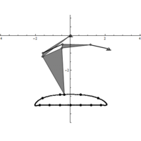
plot(X_Moment10,Y_Moment10, col = “green”, lwd = 5, xlab = “X Shift (cm)”, ylab = “Y Shift (cm)”, main = “CoG Shift By H/T Motion” )

lines(X_Moment9,Y_Moment9, col = “red” , lwd = 5)

lines(X_Moment8,Y_Moment8, col = “blue” , lwd = 5)

lines(X_Moment7,Y_Moment7, col = “cyan” , lwd = 5)

lines(X_Moment6,Y_Moment6, col = “purple” , lwd = 5)

legend(“topleft”, lty =c(1,1,1,1,1), lwd = c(1,1,1,1,1), col = c(“green”,”red”,”blue”,”cyan”,”purple”), legend = c(“R = 10cm”,”R = 9cm”,”R = 8cm”,”R = 7cm”,”R = 6cm”))

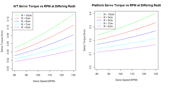
plot(MaxSpeed,2*MaxTorqueHeadX10, ylim = c(0,max(MaxTorqueHeadX10)), pch = “.”, col = “green”, xlab = “Servo Speed (RPM)”, ylab = “Servo Torque (N-m)”, main = ” H/T Servo Torque vs RPM at Differing Radii”)

lines(MaxSpeed,2*MaxTorqueHeadX9, pch = “.”, col = “red”)

lines(MaxSpeed,2*MaxTorqueHeadX8, pch = “.”, col = “blue”)

lines(MaxSpeed,2*MaxTorqueHeadX7, pch = “.”, col = “cyan”)

lines(MaxSpeed,2*MaxTorqueHeadX6, pch = “.”, col = “purple”)

legend(“topleft”, lty =c(1,1,1,1,1), lwd = c(1,1,1,1,1), col = c(“green”,”red”,”blue”,”cyan”,”purple”), legend = c(“R = 10cm”,”R = 9cm”,”R = 8cm”,”R = 7cm”,”R = 6cm”))

plot(MaxSpeed,MaxTorquePlatform10 , ylim = c(0,max(MaxTorquePlatform10)), pch = “.”, col = “green”, xlab = “Servo Speed (RPM)”, ylab = “Servo Torque (N-m)”, main = “Platform Servo Torque vs RPM at Differing Radii”)

lines(MaxSpeed,MaxTorquePlatform9, pch = “.”, col = “red”)

lines(MaxSpeed,MaxTorquePlatform8, pch = “.”, col = “blue”)

lines(MaxSpeed,MaxTorquePlatform7, pch = “.”, col = “cyan”)

lines(MaxSpeed,MaxTorquePlatform6, pch = “.”, col = “purple”)

legend(“topleft”, lty =c(1,1,1,1,1), lwd = c(1,1,1,1,1), col = c(“green”,”red”,”blue”,”cyan”,”purple”), legend = c(“R = 10cm”,”R = 9cm”,”R = 8cm”,”R = 7cm”,”R = 6cm”))

#plot(thetaLeg, LegTorque10 , ylim = c(min(LegTorque10),max(LegTorque10) + .1), pch = “.”, col = “green”, xlab = “Theta (Radians)”, ylab = “Motor Torque (N-m)”, main = “Leg Torque Versus Lever-Arm Angle”)

#lines(thetaLeg, rep(RealMaxLegTorque10, length(LegTorque)), col = “green”, lty = 2)

#lines(thetaLeg, LegTorque9 , ylim = c(min(LegTorque10),max(LegTorque9)), col = “red”)

#lines(thetaLeg, rep(RealMaxLegTorque9, length(LegTorque)), col = “red”, lty = 2)

#lines(thetaLeg, LegTorque8 , ylim = c(min(LegTorque8),max(LegTorque9)), col = “blue”)

#lines(thetaLeg, rep(RealMaxLegTorque8, length(LegTorque)), col = “blue”, lty = 2)

#lines(thetaLeg, LegTorque7 , ylim = c(min(LegTorque7),max(LegTorque9)), col = “cyan”)

#lines(thetaLeg, rep(RealMaxLegTorque7, length(LegTorque)), col = “cyan”, lty = 2)

#lines(thetaLeg, LegTorque6 , ylim = c(min(LegTorque6),max(LegTorque9)), col = “purple”)

#lines(thetaLeg, rep(RealMaxLegTorque6, length(LegTorque)), col = “purple”, lty = 2)

#legend(“topleft”, lty =c(1,1,1,1,1), lwd = c(1,1,1,1,1), col = c(“green”,”red”,”blue”,”cyan”,”purple”), legend = c(“R = 10cm”,”R = 9cm”,”R = 8cm”,”R = 7cm”,”R = 6cm”))