Introduction to LT Spice IV with Examples
Table of Contents
Purpose
The purpose of this document is to give a basic guide to getting started in using LT Spice IV SPICE simulator and show some examples of things you can do. Most of this information was compiled by experimentation and online guides which I have used in the past to develop my abilities to use this software.
SPICE simulators are extremely important in analog circuit design and are practically required for anyone interested in a Microelectronics Focus. Even if you don’t plan to focus in electronics, familiarity in a SPICE simulator will enrich your learning experience for required analog electronics courses (EE330 & EE430) and is handy for design problems you may face at some point in your career.
This is by no means a comprehensive guide, and is only for introduction and basic circuit construction purposes. This guide provides a cursory overview of basic use of the software, and should allow you to explore its capabilities with some confidence. This is the tip of the iceberg when it comes to using circuit simulation tools, and hopefully will get you to the point where you can start learning comfortably on your own.
What is LT Spice IV?
I think that Linear Technologies, maker of LT Spice IV, gave a great description of the program on their download page:
LTspice IV is a high performance SPICE simulator, schematic capture and waveform viewer with enhancements and models for easing the simulation of switching regulators. Our enhancements to SPICE have made simulating switching regulators extremely fast compared to normal SPICE simulators, allowing the user to view waveforms for most switching regulators in just a few minutes. Included in this download are LTspice IV, Macro Models for 80% of Linear Technology’s switching regulators, over 200 op amp models, as well as resistors, transistors and MOSFET models.
SPICE Simulators are very powerful tools for circuit analysis. It also functions as a great schematic editor if you just need to draw up a general schematic for your project or for a technical report. Learning to use a SPICE Simulator is especially useful for classes with analog electronic circuit analysis (EE330 & EE430).
LT Spice IV differs from other Spice simulators in that it was developed by and populated with Linear Technology devices. You can import external libraries to add a specific part using generic Spice files easily if you need to make a specific simulation with parts you have specced in advance.

Example of some Default-Modeled LT Components
After opening LT Spice, you can start a new schematic or open an existing one. To start a new schematic press the new schematic button in the upper left of the window:
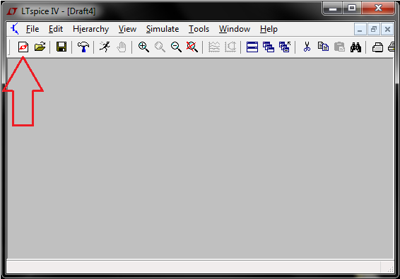
Initial Window after Opening LT Spice IV
Starting a new schematic creates a blank area where you can start building a schematic for analysis and design. You can also highlight the grid by pressing Ctrl-G. You can zoom in an area using the magnifying tools in the toolbar or by using the mouse wheel.
On the Windows version, there are dozens of buttons on the toolbar and this guide will go over the useful ones throughout the next steps concerning building a basic circuit. In the Mac version, you will have to rely elsewhere.
Building a Circuit
These are the basic tools on the toolbar along the top of the Schematic Editor. They can all be accessed with hotkeys which are intuitive for common components: (R) Resistor, (L) Inductor, (C) Capacitor, (G) Ground, (D) Diode.
![]()
Circuit Building Toolbar
Less obvious is the Component ![]() button (F2) which opens a vast catalog of available parts and systems which are included by default with LT Spice IV. You can search for parts by name or by clicking the [categories] on the left.
button (F2) which opens a vast catalog of available parts and systems which are included by default with LT Spice IV. You can search for parts by name or by clicking the [categories] on the left.
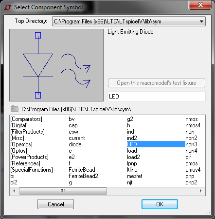
Example: Selecting Components from Component Catalog
The Draw Net![]() (F3) button allows you to draw connections (nets) between components. This turns the cursor into a dashed crosshair to help align nets and keep things organized. In the scope of the schematic, these nets are like ideal wires with zero impedance. Start by pressing CTRL-G to show the grid, place two resistors (R), and a few nets to connect them in series.
(F3) button allows you to draw connections (nets) between components. This turns the cursor into a dashed crosshair to help align nets and keep things organized. In the scope of the schematic, these nets are like ideal wires with zero impedance. Start by pressing CTRL-G to show the grid, place two resistors (R), and a few nets to connect them in series.
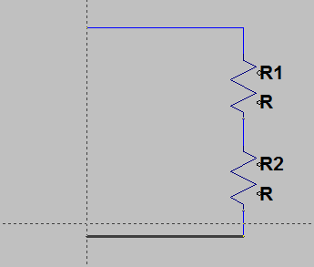
Circuit Under Construction
After placing a component with properties such as resistance, the values will need to be set if you plan to run a simulation. To set this property, right-click the component and enter a value. LT Spice IV supports some shorthand notations for value magnitudes such as Kilo and milli by placing the letter after the number (ex. 100n = 100e-9 = 0.1u).
| Spice Shortcut | Alternate | Short For | Value |
| 10 t | 10e12 | tera | 10 000 000 000 000 |
| 10 g | 10e9 | giga | 10 000 000 000 |
| 10 meg | 10e6 | mega | 10 000 000 |
| 10 k | 10e3 | kilo | 10 000 |
| 10 | 10e0 | – | 10 |
| 10 m | 10e-3 | milli | 0.010 |
| 10 u | 10e-6 | micro | 0.000 010 |
| 10 n | 10e-9 | nano | 0.000 000 010 |
| 10 p | 10e-12 | pico | 0.000 000 000 010 |
| 10 f | 10e-15 | femto | 0.000 000 000 000 010 |
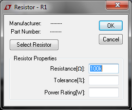
Right-Click Menu of a Resistor
For most components, you have the option of choosing a predefined part. This allows you to model specific components that you have chosen to use and can be very useful when designing an analog circuit for real-world use. If you do not select a specific part (ex. LM741 Op-Amp), most components placed will act ideal by default (no ESR or parasitic capacitance).

Example: Window for Selecting a Specific Model of Diode
Linear Technologies has a handy guide for importing third-party devices which can be found here: http://www.linear.com/solutions/1083
Important Default Hotkeys
These are a few of the important default hotkeys that you will use constantly when working in LT Spice. Some hotkeys are only available in the Windows version of LT Spice, and Mac versions may need a simple workaround (ex. on Mac, R does not create a resistor, and it must be placed by finding it in the F2 catalog window). Windows-only defaults are marked with an asterisk (*).
| Shortcut | Symbol | Function | Description |
| F2 | Component Catalog | Open component catalog for selecting | |
| F3 | Draw Net | Draw wires between components | |
| F4 | Create Port | Create a port for naming nodes in the circuit or create a ground | |
| F5 | Delete | Click on a component or wire to delete, or drag an area to delete objects in the area | |
| F6 | Copy | Click an element or wire to create a copy of it or drag to copy a group of parts | |
| F7 | Grab | Grab and move an element, disconnects from circuit. Drag to select multiple parts. | |
| F8 | Drag | Grab and move an element, keeps current connections. Drag an area to select multiple parts | |
| F9 | Undo | Undoes previous action | |
| G | Ground | Create Ground node | |
| R* | Resistor | Place a resistor | |
| C* | Capacitor | Place a capacitor | |
| L* | Inductor | Place an inductor | |
| D* | Diode | Place a diode | |
| Ctrl-R | Rotate | Rotate part 90 degrees clockwise | |
| Ctrl-E | Mirror | Flip part horizontally | |
| T | Text | Place text (for documentation/notes) | |
| S | SPICE Directive | Place SPICE directive |
Changing Default Hotkeys
You can also easily change or get an overview of the default hotkeysby pressing the Control Panel button ![]() (or Tools > Control Panel), navigating to the Drafting Options tab, and pressing the Hot Keys button.
(or Tools > Control Panel), navigating to the Drafting Options tab, and pressing the Hot Keys button.
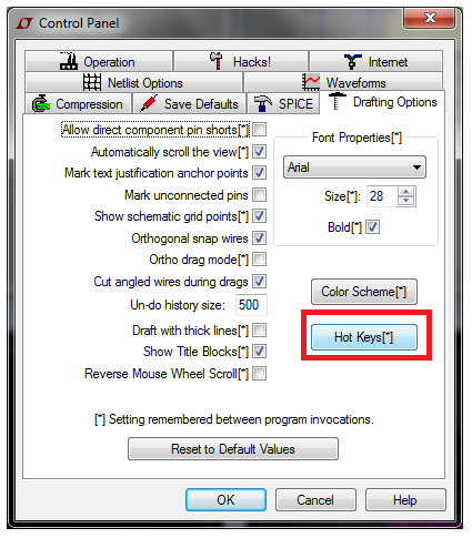
Navigation to Edit Hotkeys Window
Voltage & Current Sources
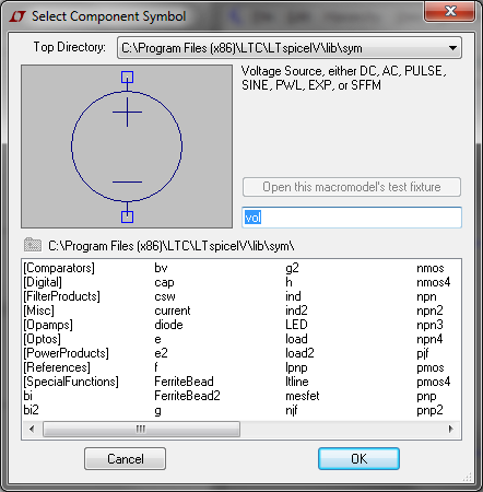
Voltage and Current sources can be added to your design by selecting them in the Component Symbol window (F2). A general purpose voltage source can be found by searching for “vol” in the text search bar as shown below:
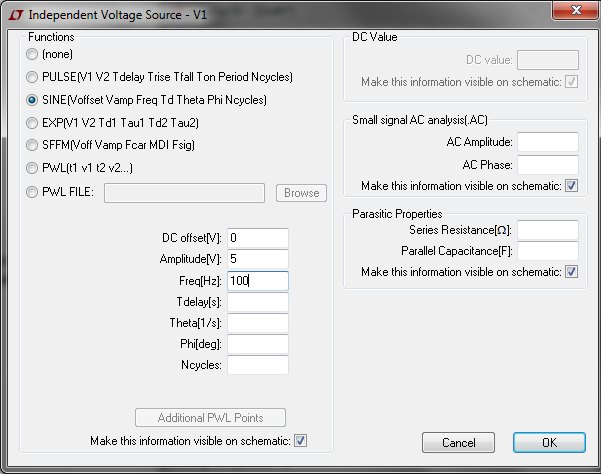
By default, sources are ideal DC sources, but can be given advanced settings to create an AC signal such as a PWM or sinusoid waveform. To do this, right-click the source once it has been placed and click Advanced.
Running a Simulation
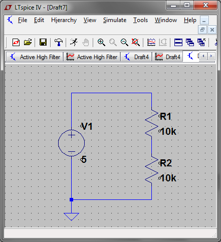
Before running a simulation, all of the components and sources should be given values, and a ground node (G) must be declared and connected to the circuit. For this simple example, the circuit should look like what is shown below.
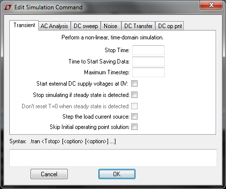
Pressing the run simulation ![]() at this point will bring up the simulation configuration window where you can edit the type of simulation. The default and most simple simulation is a transient analysis where the circuit is simulated for a determined period of time.
at this point will bring up the simulation configuration window where you can edit the type of simulation. The default and most simple simulation is a transient analysis where the circuit is simulated for a determined period of time.
After running the simulation and setting a stop time for a transient analysis, a blank plot pane will open with your specified time period on the x-axis. You can now click on the circuit in different locations to get information on the voltage, current, and power at specific nodes and components.
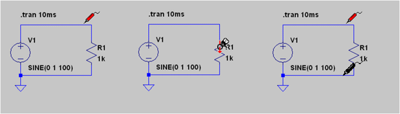
Below are three examples of locations you can click to get information on the circuit
- Left-click on net: Clicking on a net will give you the voltage with respect to ground at that node as a function of time on the plot pane.
- Left-click on component: Clicking directly on a component will give you the current through the component as a function of time.
- Click-drag between nets: Clicking on a node and dragging to another node will give you the voltage between those nodes.
Not shown above are a few other probes you can use with shortcuts:
- Alt-Click on component: This will display the power dissipation of a component (cursor turns into a thermometer)
- Alt-Click on a net/wire: Show current through the net (cursor turns into a multimeter with arrow)
- Multiport Devices: For components such as transistors where there are more than two nodes, you can click right where it connects to the circuit to see individual currents
Clicking different locations will add more plots to the pane so they can be analyzed easily. To remove nets you can right-click the plot or simply double-click a probe area on the schematic to isolate it’s plot and remove others.
Basic Spice Directives
After running the simulation, you may have noticed that there is some black text placed on the schematic that says .trans 10 or whatever you set the stop time to be. This is a SPICE directive and can be used to do things such as set variable values and create step parameters. You can edit these directives by right-clicking on them.
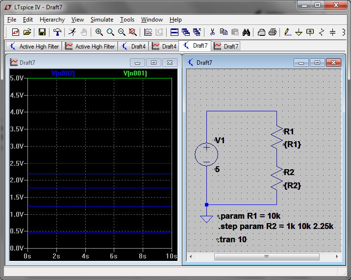
Below is an example where the resistor values for R1 and R2 were set by variables named R1 and R2 respectively. In order to use a variable value you must set the component values between {curly brackets} or the simulation will not run. You can also use math operations as long as they are within the curly brackets (ex. {15*(R1*R2)/(R1+R2)}).
In this example, .param R1 = 10k is pretty self-explanatory and it will set the parameter R1 to 10k. Less obvious is the use of the command .step param R2 = 1k 10k 2.25k. This creates a step parameter and will run the simulation for each step in the setup. This command says that R2 should vary from 1k to 10k with a step size of 2.25k, creating 5 simulations with the separate values (1k, 3.25k, 5.5k, 7.75k, 10k). The plot pane shows the source voltage (green) and the voltages at R2 for the 5 simulations run (blue).
DC Sweep (Linear Regulator)
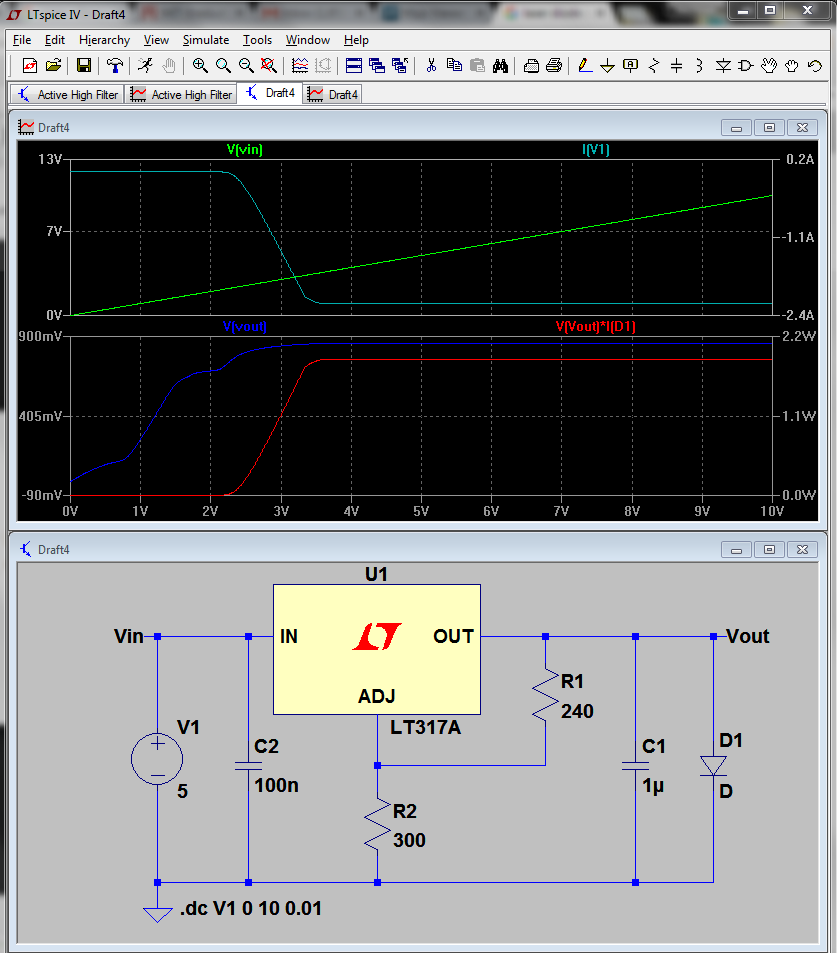
This is an example of using one of the predefined subsystems (linear voltage regulator) and a linear DC sweep simulation. The top plane is a plot of source voltage (green, scale on left), versus source current (increases from about 0A to over -2A as the regulator becomes active, scale on right).
The bottom plane shows the diode voltage (blue, scale on left) and the diode power dissipation (red, scale on right.
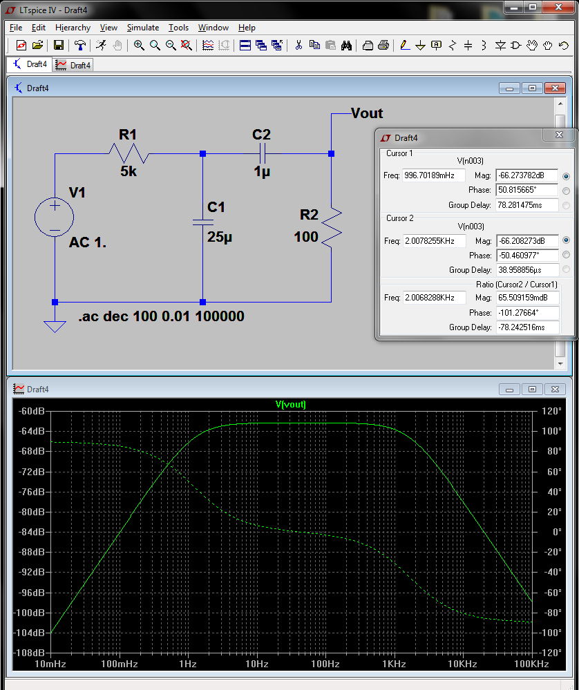
AC Analysis (Second-Order Bandpass Filter)
This is an example of using a simple second-order RC bandpass filter and an AC analysis. The resultant plot is essentially a Bode plot of the output voltage with respect to the input voltage.
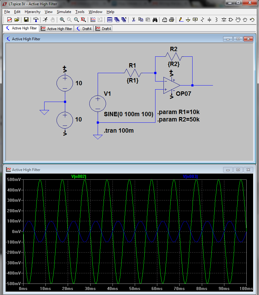
Transient Analysis (Inverting Amplifier)
This is an example of using an ideal simulated Op-Amp (OP7) to create an inverting amplifier. This was taken from EE430 Lab Manual and shows a transient analysis of an inverting amplifier with Av gain of -5.
Note the port name and connections to create the positive and negative DC source voltages for the Op-Amp and location of ground nodes.
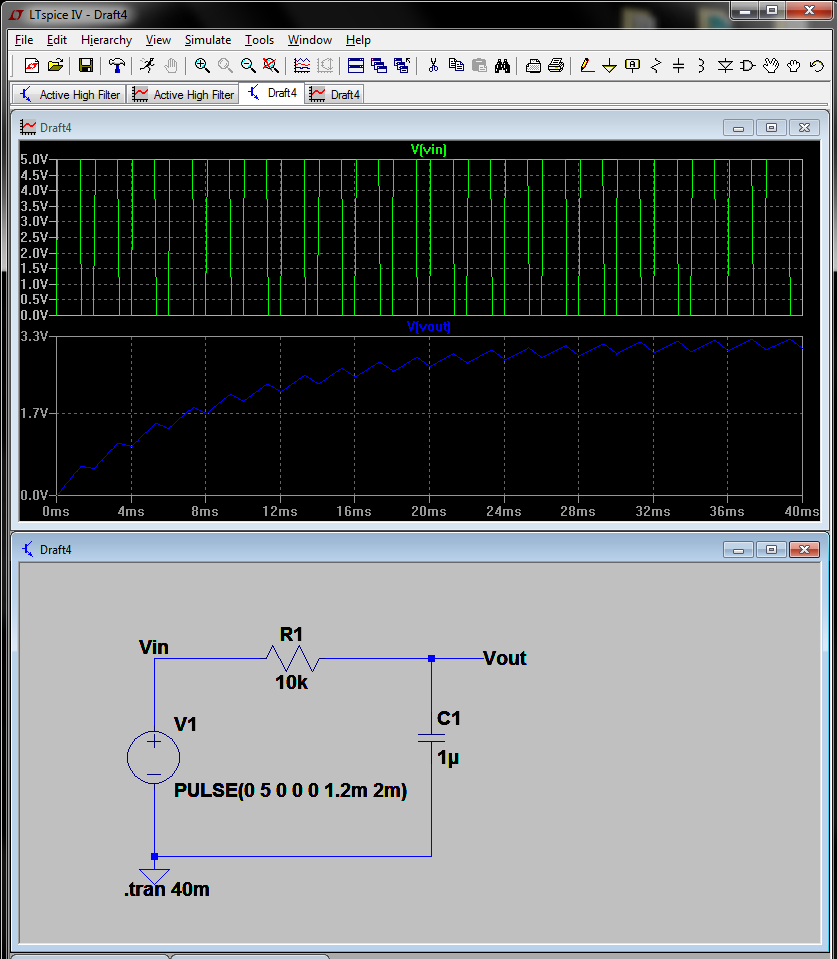
Transient Analysis (PWM Filtering)
This is an example adapted from the training series on Arduino Analog I/O on the subject of PWM filtering. The voltage source was set to produce a 500Hz PWM signal with duty cycle of 60% and amplitude of 5v (top plot). After the low pass filter at Vout (lower plot), it can be seen that there is a small ripple voltage, and the higher frequencies are filtered out to leave a DC voltage of roughly 3.0v (60% of 5v).
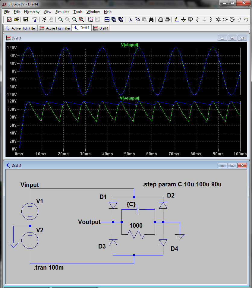
Step Parameter (Full-Wave Bridge Rectifier)
This is an example of a full-wave bridge rectifier (EE330) which converts a center-grounded AC signal of 120v amplitude and frequency of 60 Hz (top plot) into a rectified output of roughly 120v DC. This example also uses the step parameter directive to show the effects of using a 10uF filter capacitor (green, high ripple voltage) and a 100uF filter capacitor (blue, lower ripple).